

By: Hetansh Gosar
The buying and selling technique focuses on hole buying and selling in Indian equities, particularly focusing on shares with decrease volatility and avoiding high-volatility market situations. This long-only method includes coming into positions on the day’s shut and exiting on the subsequent day’s open. As Indian markets mature and extra shares turn out to be eligible for buying and selling, the technique’s efficiency improves over time, yielding higher outcomes and a better Sharpe ratio. Hole buying and selling gives better predictability and considerably reduces volatility, making it a dependable and efficient method for constant returns.
This text is the ultimate undertaking submitted by the creator as part of his coursework within the Govt Programme in Algorithmic Buying and selling (EPAT) at QuantInsti. Do test our Tasks web page and take a look at what our college students are constructing.
Different EPAT Undertaking publications on Hole Buying and selling Technique and Markov Rule are listed beneath:
In regards to the Writer
My title is Hetansh Gosar, a 23-year-old from Ahmedabad. I maintain a Bachelor’s diploma in Enterprise
Administration and have efficiently accomplished all three ranges of the Chartered Market Technician (CMT) program. I shall be eligible for the CMT constitution upon finishing three years of business expertise. For the previous two years, I’ve been working as a Technical Researcher, gaining useful experience in market evaluation and buying and selling methods.
EPAT batch: #61Certification standing: Certification of Excellence Mentor: Rekhit Pachanekar
Join with me: www.linkedin.com/in/hetansh-gosar
Technique Thought
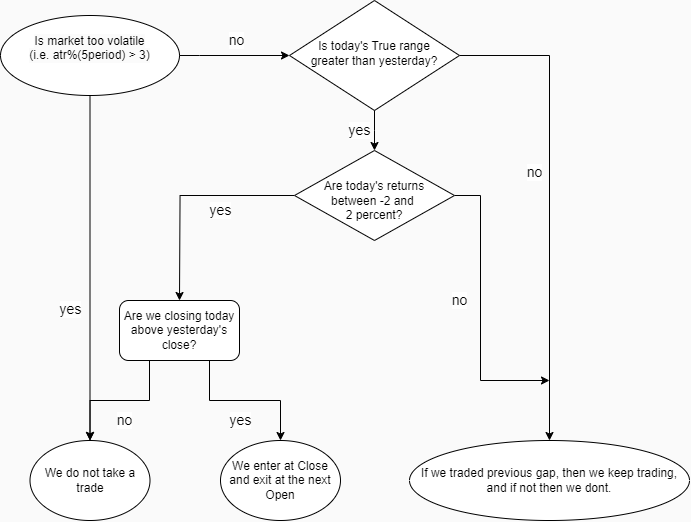
The concept is to enter the market when the situations are glad:
If at this time’s candlestick physique is bigger than yesterday’s candlestick physique (that is to point a rise in momentum).If at this time’s shut is bigger than the open (that is to point a optimistic momentum).At present’s proportion change ought to be lower than 2%(with a view to keep away from trades throughout excessive volatility such because the Nice Recession or COVID-19).If these three situations are glad then we enter on at this time’s closing and exit on the following day’s opening. The graph reveals the parameters of when to take a commerce.
Motivation
The motivation for the technique comes from the concept a powerful momentum that continued throughout the day would proceed even when the markets had been closed and never being traded. Therefore there could be a spot within the opening of the following day. We wish to seize that hole by coming into proper earlier than the shut and exiting on the open. We use lengthy trades solely as in case of up strikes, there may be predictive energy of the day prior to this, whereas not the identical with down strikes.
As there isn’t a certainty of continuation in pattern in case of down strikes, there may be a change of sentiment and we cannot have the ability to seize the hole. We use the true vary of candles because the true vary can present us what the intrinsic power of the day was.
When there is a rise within the dimension, we will decide that the momentum has elevated for the day which might imply a powerful sufficient momentum. When there may be an excessive amount of volatility in markets, comparable to throughout the crash of COVID-19 or the good recession, the predictive energy of the day prior to this is misplaced and there’s a lot of pointless motion out there.
To keep away from that, we don’t take trades which are better than 2% in closing as that may be lots of volatility, and likewise with such nice returns on the day of entry, there are possibilities of a little bit of retracement on the following day. By utilizing simply gaps to commerce, we don’t get lots of returns and lots of returns, however we get extra secure returns. We will use leverage to enlarge the returns, and we aimed to have a better-adjusted hit ratio, so we may have a smoother fairness graph.
Undertaking Summary
The technique is designed in a method that targets the commerce hole. It generates an entry on closing and the exit is on the subsequent open. This technique finest works for low-volatility shares (equities with much less ATR/worth ratio) in Indian markets.
The findings recommend that there was an honest revenue with much less volatility, theoretically, in backtesting.
Dataset
We use nifty each day knowledge as our buying and selling dataset.
Knowledge Mining
The information we’re utilizing is of the inventory itself and nifty knowledge together with it. The technique requires inventory knowledge for coming into at shut worth, exiting at open worth, and excessive, low and shut knowledge for ATR. Whereas nifty knowledge is required for its ATR since we have now used a filter through which if the market is extraordinarily risky, we keep money and don’t commerce.
The information is downloaded from yfinance, which is part of the code of the testing technique itself. So, when the perform of the backtesting technique is run, each the information (nifty and inventory) shall be downloaded after which the backtesting will happen.
After the backtesting is completed, there’s a completely different set of code which is of pyfolio, run to have outcomes.
The coding is completed in Python utterly.
The ten shares used to create a portfolio are:
Bharti-airtelCoal IndiaColpalLTM&MRelianceSBISolaris IndsTrentZydus Lifescience
The testing was finished over a interval of 10 years, from 2014-1-1 to 2024-1-1. It doesn’t make sense to check earlier than a sure variety of years, for the reason that markets had been very risky again then, however had ultimately turn out to be much less risky. As our markets are maturing, there are increasingly shares turning into much less risky and they’d then be tradable.
Knowledge Evaluation
What we came upon is that often shares gave an honest return, often better than 15% CAGR, with round a max drawdown of 10 to fifteen per cent.
If we create a portfolio of the ten shares talked about above, the CAGR comes out to be round 24.9%, cumulative returns 771.6%, annual volatility round 4.1%, and max drawdown round 2.4%.
Key Findings
The technique works nicely when the markets are in a low volatility part. The shares ought to be basically low risky and never essentially up trending. This technique works finest in a portfolio, as there may be not a lot systematic threat and extra unsystematic threat, so when buying and selling an entire portfolio, the risk-adjusted returns are fairly robust. The theoretical sharp ratio is popping out to be greater than 5, which is due to extraordinarily low volatility, but it surely must be examined in dwell markets as there are a number of limitations of the technique as nicely.
Challenges/Limitations
One of many biggest challenges is to get the open worth, because the technique is examined on previous knowledge, we have now a transparent opening worth, however we have to seize the opening worth with a view to get the very same outcomes.
The transaction prices usually are not included within the backtest outcomes, which could possibly be fairly excessive as we enter and exit trades on an on a regular basis foundation.
Conclusion
The technique theoretically works nicely. It has adequate returns for the quantity of threat we take. The constraints may be essential and ought to be thought of as they might skew the outcomes drastically. But when there may be not a lot change in returns, and due to the low volatility, we’d nonetheless have the ability to get a decently or well-performing technique after utility. A advantage of this technique is that it’s utilized to fairness, so we don’t face challenges of derivatives, and as time goes by, and markets mature, the pool of shares for us to select from will increase, so we will deploy extra capital in it with much less influence price.
This technique may be good for somebody searching for a average return with much less threat. For somebody keen to threat extra and bear the expense of curiosity, getting leverage is an choice. The technique has secure returns particularly in portfolio format so taking leverage shouldn’t be that tough. With the CAGR of the portfolio being round 25%, it did beat the index nicely, additionally with a lot lesser volatility. It doesn’t have an effect on a lot if the markets usually are not bullish, it would create some volatility in our portfolio returns however may not face large drawdowns.
Annexure
The next is the code used to generate the technique perform used to create a “pandas” dataframe with technique returns in it:
def technique(inventory,start_date,end_date):
# Downloading knowledge
df1 = yf.obtain(inventory, begin = start_date, finish = end_date, auto_adjust = True)
knowledge = yf.obtain(‘^NSEI’, begin = start_date, finish = end_date)
# Creating ATR and volatility filter on nifty
knowledge[‘atr’] = ta.ATR(knowledge[‘High’], knowledge[‘Low’], knowledge[‘Close’], 5)
knowledge[‘atr_perc’] = knowledge[‘atr’]/knowledge[‘Close’]
# Merging knowledge of nifty and inventory
df = df1.merge(knowledge[[‘atr_perc’]], left_index=True, right_index=True, how=’left’)
# Creating returns
df[‘returns’] = np.log(df[‘Close’]/df[‘Close’].shift())
# Creating true vary
df[‘true_range’] = np.most.cut back([df[‘High’]-df[‘Low’],
df[‘High’]-df[‘Close’].shift(),
df[‘Close’].shift()-df[‘Low’]])
# Creating situations of entry
df[‘condition’] = np.the place( (df[‘true_range’] > df[‘true_range’].shift()) &
(df[‘returns’] < 0.02) &
(df[‘returns’] > -0.02), 1, 0)
# Creating sign with the assistance of situation
df[‘signal’] = np.nan
df[‘signal’] = np.the place((df[‘condition’] == 1) & (df[‘returns’] > 0), 1,
np.the place((df[‘condition’] == 1) & (df[‘returns’] < 0), 0, np.nan))
df[‘signal’] = df[‘signal’].ffill()
# A filter for avoiding risky intervals
df[‘signal’] = np.the place(df[‘atr_perc’].shift() > 0.03, 0, df[‘signal’])
# Calculating the returns on buying and selling the hole
df[‘o_c_returns’] = np.log(df[‘Open’]/df[‘Close’].shift())
# getting returns
df[‘strategy_returns’] = df[‘signal’].shift() * df[‘o_c_returns’]
df[‘cum_strategy_returns’] = df[‘strategy_returns’].cumsum()
df[‘b&h_returns’] = df[‘returns’].cumsum()
return df
File within the obtain
The Python codes for implementing the technique are offered within the downloadable button together with knowledge obtain, code used to generate the technique perform used to create a “pandas” knowledge body with technique returns in it.
Login to Obtain
Subsequent Steps for you
Wish to know the way EPAT equips you with abilities to construct your buying and selling technique in Python? Take a look at the EPAT course curriculum to search out out extra.
Hole Buying and selling Technique is among the easiest buying and selling methods for day merchants. Take a look at the course on Day Buying and selling Methods for Newbies if you’re involved in day buying and selling.
If you’re involved in studying extra about Hole Buying and selling and Markov Rule, learn the blogs right here:
Discover EPAT buying and selling initiatives on varied matters:
Disclaimer:The knowledge on this undertaking is true and full to one of the best of our Scholar’s information. All suggestions are made with out assure on the a part of the coed or QuantInsti®. The scholar and QuantInsti® disclaim any legal responsibility in reference to the usage of this data. All content material offered on this undertaking is for informational functions solely and we don’t assure that by utilizing the steering you’ll derive a sure revenue.


